Estimated rows and actual rows

SQL Server calculates how many rows it expects at each operator and, when we capture an actual plan, records how many it observed during that execution. Comparing both figures helps locate an assumption that did not match the data found.

Where they appear in SSMS

Enable Include Actual Execution Plan with Ctrl+M, run the query, and open the Execution plan tab. Then place the pointer over an operator. SSMS displays a card with its properties; you can also select it and press F4 to inspect them in the Properties window.

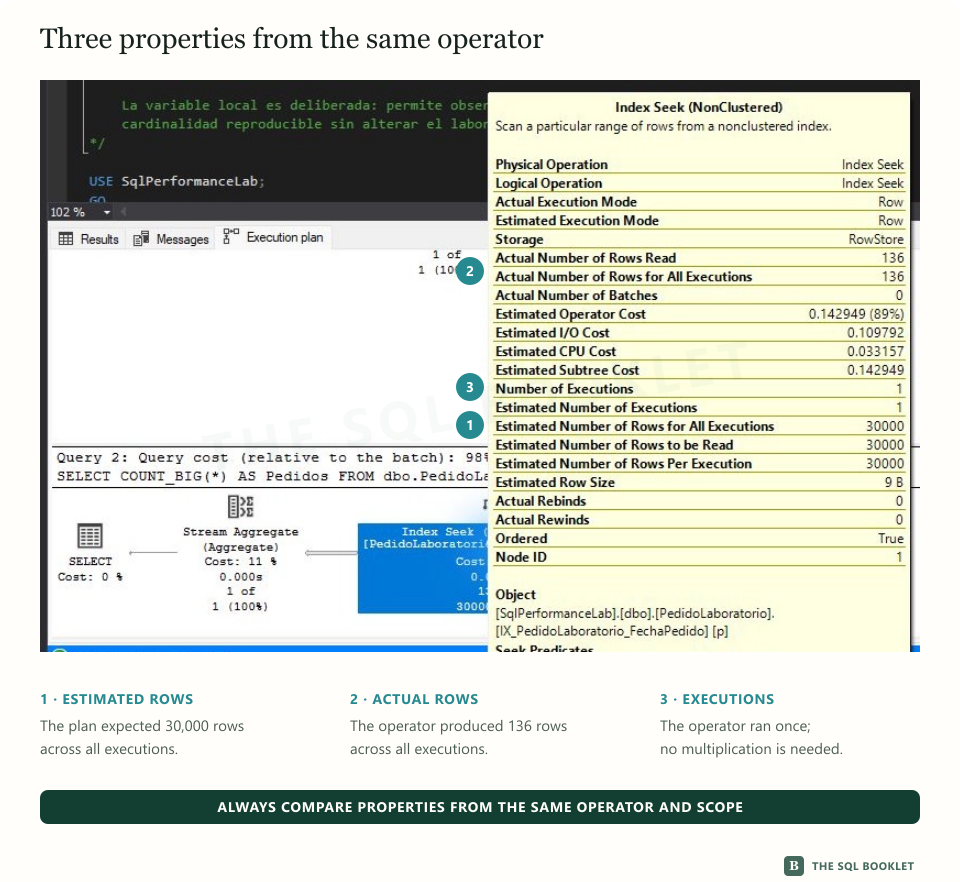
The screenshot shows an Index Seek selected in blue. Markers 1, 2, and 3 identify the three properties needed for this reading:

• Estimated Number of Rows For All Executions: 30000;
• Actual Number of Rows For All Executions: 136;
• Number of Executions: 1.

The estimated and actual values belong to the same operator and cover all its executions. In this case the operator ran once, so we can compare 30000 with 136 without applying another multiplication.

Two figures from two moments

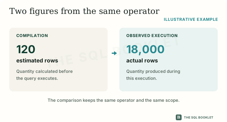
Estimated rows are the quantity calculated by the optimizer during compilation. This calculation is part of cardinality estimation: predicting how many rows an operation will produce at one point in the plan.

Cardinality is a row count. The plan contains an estimate for each operator because the output of one operation becomes the input of the next.

Actual rows are the rows produced by the operator during the observed execution. They appear only when the query ran and execution information was captured, as in an actual execution plan.

“Actual” does not mean permanent or universal. It describes what happened with those data, parameters, and conditions. Another execution may produce a different quantity.

The comparison belongs to the same operator

We must compare the estimated and actual values of the same operator. Comparing the estimate of one input with the actual rows of another branch mixes different points in the plan.

We also need to preserve the same scope. Properties may present values per execution, accumulated across all executions, or distributed among several threads. Before calculating a difference, check:

1. the complete name of each property;
2. the operator execution count;
3. whether the figure already covers all executions;
4. whether a per-thread breakdown exists.

If a value already represents all executions, multiplying it by the execution count again would duplicate the quantity.

Three relationships we may find

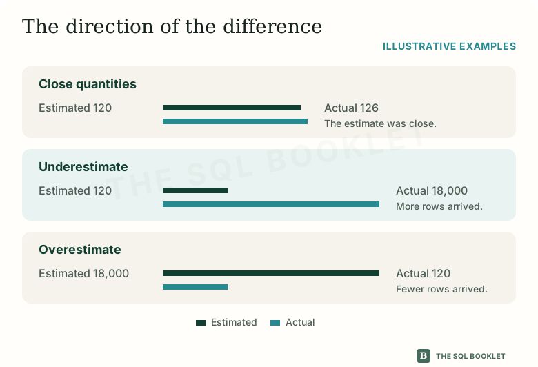
When the quantities are close, the estimate described that part of the execution reasonably well. They do not have to be identical to be useful.

An underestimate occurs when the operator produces many more rows than expected. SQL Server prepared that part of the plan for a smaller input than the one observed.

An overestimate occurs when the operator produces many fewer rows than expected. The plan was prepared for a volume that did not appear in that execution.

These names describe the direction of the difference. They do not yet explain its cause or prove that the operator must be changed.

Why the difference deserves attention

The optimizer uses estimated cardinality as an input to its cost model. It uses that model to compare access methods, join strategies, operation order, and memory needs.

If a branch supplies a very different quantity, downstream operators receive a volume unlike the one considered during compilation. The difference can propagate: an inaccurate estimate near the beginning of a branch can influence several later decisions.

The effect does not depend only on how far apart the figures are. It also matters where the difference begins, how many operators receive it, how often they execute, and what work they perform with those rows.

This is why we do not adopt a universal rule such as “ten times is a problem.” A large difference may have little impact in a small branch, while a smaller difference may accumulate inside a repeated operation.

Questions raised by a difference

A substantial separation lets us formulate specific questions:

• do the statistics describe the current data distribution?;
• does the requested value occur with an unusual frequency?;
• does the parameter used during compilation represent this execution?;
• does the predicate contain an expression, variable, or function that limits the information available for estimation?;
• does the difference begin at this operator or arrive from an earlier input?;

Statistics summarize how selected values are distributed. Distribution describes how frequently values occur: some may repeat often while others appear rarely. The optimizer uses this information, together with other rules, to approximate how many rows will satisfy a predicate.

These questions are investigation hypotheses. A difference between estimated and actual rows does not authorize us by itself to update statistics, create an index, recompile a procedure, or rewrite the query.

Separate observation, hypothesis, and verification

A careful reading can be documented like this:

• Observation: the operator estimated 30,000 rows and produced 136 in this execution.
• Hypothesis: distribution, statistics, the parameter, or the predicate might explain the difference.
• Pending verification: locate where the separation begins and inspect the corresponding evidence before proposing a change.

This form keeps visible what we know and what we still need to demonstrate.

What this still does not establish

A close estimate does not prove that the query is fast. A distant estimate does not prove by itself that the query is slow or that the difference is the main cause of the observed symptom.

To assess the impact, we still need to relate the quantities to rows read, executions, predicates, memory, reads, CPU, and duration. The plan provides a signal; measurement and context determine how much it matters.

Reasonable next check

The next entry distinguishes Index Seek, Index Scan, and Table Scan. There we will relate the access method to rows read, rows returned, and the applied predicate.