
How an execution plan tree is organized
An execution plan may extend from left to right on the screen, but its structure is described as a tree. Recognizing its parts lets us follow the strategy without relying yet on the meaning of every icon.
Why it is considered a tree
A tree organizes elements through relationships between a main point and the elements that contribute information toward it. In a plan, one operation can receive rows produced by one or more earlier operations.
Each element in the tree is a node. In SQL Server plans, a node represents an operator: a task that obtains, transforms, or returns rows.
Connections between nodes show which operator supplies rows to the next one. The complete plan brings those relationships together until it produces the requested result.
The root operator
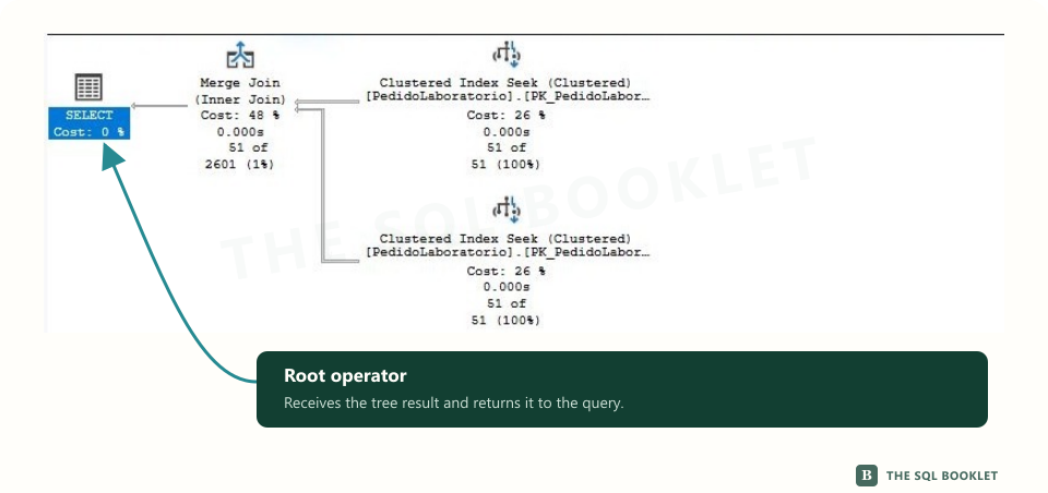
The root is the point where the tree ends. In a simple graphical plan, it usually appears on the left and represents delivery of the final result.
The root operator does not necessarily perform most of the work. Its position tells us that it receives the result produced by the rest of the tree. To understand where that result comes from, we follow its connections toward the operators that feed it.
Entry points
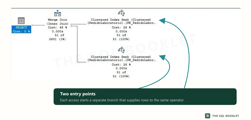
At the opposite end are operators that begin obtaining rows from a table, index, or another source. We can treat them as entry points when beginning to read a branch.
A branch is a path made of connected operators that prepare an input for another operator. It may contain a single access operation or several filtering, calculation, sorting, or aggregation tasks.
When an operation needs two sets of rows, the tree shows two branches reaching the same node. Each branch may have obtained and prepared its data differently.
Arrows represent flow
Arrows connect operators and point in the direction rows move. Following them lets us reconstruct what information each task receives and which operation receives its output.
Row flow means the logical movement of results between operators. It does not imply that every row must exist as a complete set before moving forward. Some operations can return rows while other parts of the plan continue working.
Arrow thickness, row counts, and execution counts add more information. To reconstruct the tree first, follow the connections between operators.
How to follow flow through the plan
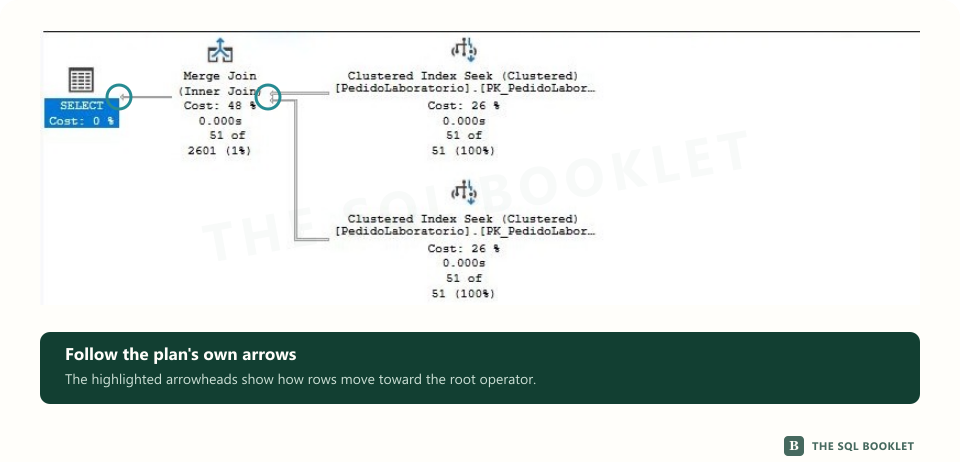
In SQL Server graphical plans, it is often useful to begin with operators on the right and follow the arrows toward the left. When several branches exist, we can trace each input before continuing toward the node where they meet.
This orientation is not an exact chronology. SQL Server can request rows between operators, interleave work, and use parallelism. The diagram explains producer-and-consumer relationships between rows, not a rigid sequence in which one step must finish before the next begins.
Parallelism means that SQL Server can distribute part of the work across several execution threads. Its operators do not turn horizontal position into a measure of elapsed time either.
Describe the tree before evaluating it
Before deciding whether a plan contains a problem, we can describe only its structure:
- locate the root operator;
- identify how many inputs it receives;
- follow each branch to its entry points;
- recognize where rows meet or change;
- return to the flow that leads to the result.
This description separates observation from diagnosis. Knowing how to traverse the tree does not yet mean that we know whether its choices are appropriate.
What this still does not establish
The shape of the tree explains how operators relate, but it does not prove which branch consumed the most time or which one should change. Position, icon size, and visual order do not replace properties and measurements.
We should not assume that the first operator that attracts our attention caused the problem. First we reconstruct the flow; later we examine quantities, execution counts, conditions, and observed work.
Reasonable next check
The next article studies arrows, properties, and execution counts. With that vocabulary, we can move from the general shape of the tree to the evidence associated with each operator.