
Arrows, properties, and execution counts
An execution plan diagram lets us recognize operators and connections, but its visible labels do not contain all the evidence. Arrows provide an initial orientation; properties let us verify which quantity they represent and how many times each operator participated.
What an arrow indicates
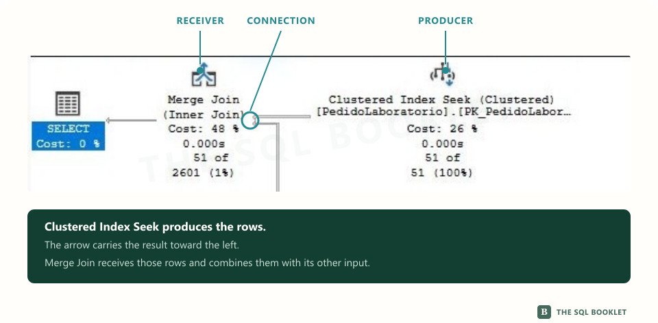
An arrow shows that one operator supplies rows to another. In a SQL Server graphical plan, it points from the operator that produces the rows toward the operator that receives them. This is why row flow is usually followed from right to left until it reaches the root.
Each connection identifies which operator receives the result and lets us inspect how many rows passed through it.
In the screenshot, Clustered Index Seek is the producer because it supplies rows. Merge Join is the receiver because it uses them as one of its inputs. The arrowhead sits next to the receiver and reveals the direction of row flow.
Work is requested in the opposite direction from row flow. This model is known as demand-driven execution: an operator does work when another operator asks it for data, without requiring every box to finish completely before the next one begins.
Thickness represents relative volume
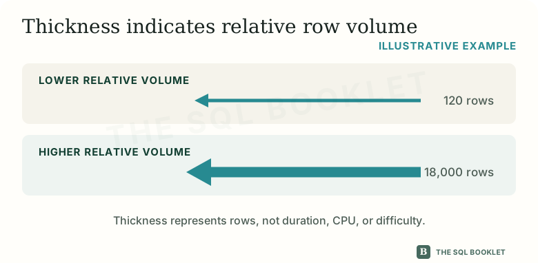
A thicker arrow draws attention to a larger row quantity associated with that connection. It helps locate parts of the plan that transport more data, but it remains a visual representation.
Thickness does not represent duration, CPU, or difficulty. A thin arrow can belong to an expensive operation, while a thick arrow may move rows with little work per row.
We should not derive an exact number from appearance alone. To learn which quantity the diagram uses —estimated or observed— we must open the properties and identify the plan mode.
The visible cost is still an estimate
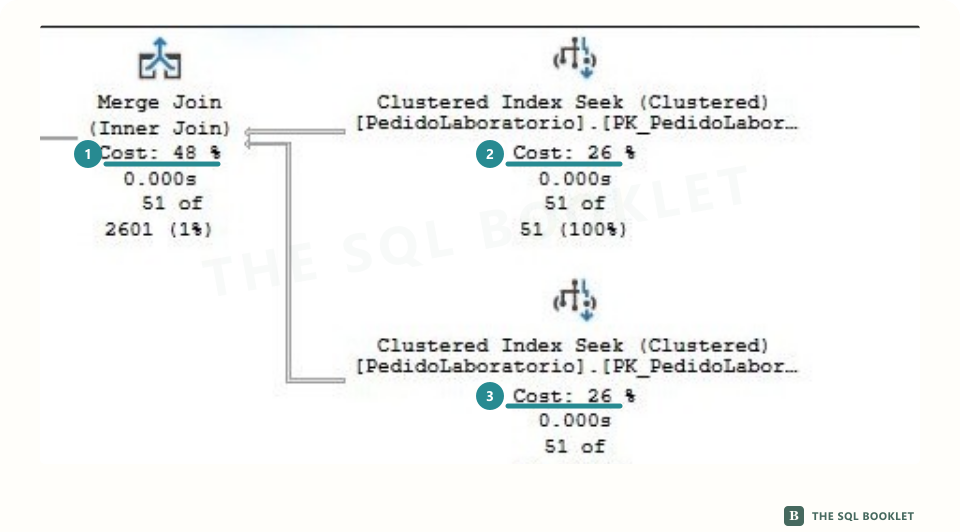
- 1Merge Join
Represents 48% of the estimated cost.
- 2Clustered Index Seek
Represents 26% of the estimated cost.
- 3Clustered Index Seek
Represents the remaining 26%.
An operator label may show a cost percentage. That percentage comes from the model the optimizer uses to compare alternatives. It is not the percentage of elapsed time or CPU consumed during execution.
In the screenshot, the Merge Join represents 48%, while each Clustered Index Seek represents 26%. Together they make up 100% of that statement’s estimated cost; they describe how the model distributed cost, not how long each operator ran.
We must also distinguish two scopes:
- the cost of a statement is compared with the other statements in its batch;
- the cost of an operator is presented within that statement’s plan.
Percentages help us navigate the same estimated context. They do not turn operators from separate queries into directly comparable measurements.
The tooltip brings key properties together
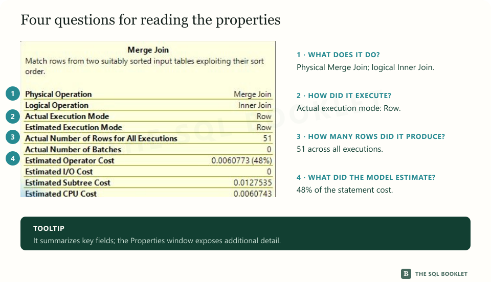
The screenshot shows an operator tooltip. This summary exposes several properties without leaving the plan; the Properties window offers additional fields whose names and availability can vary with the operator, the plan mode, and the tool version.
Useful fields to locate include:
- physical and logical operation;
- the referenced object, when one exists;
- predicate or seek predicate;
- estimated rows;
- actual rows, when the query executed;
- actual number of executions;
- warnings and values associated with the operator.
One property rarely provides enough context. The object tells us where the operator works; the predicate, which condition it applies; the rows, how much output it produces; and the execution count, how often that participation repeats.
What the execution count measures
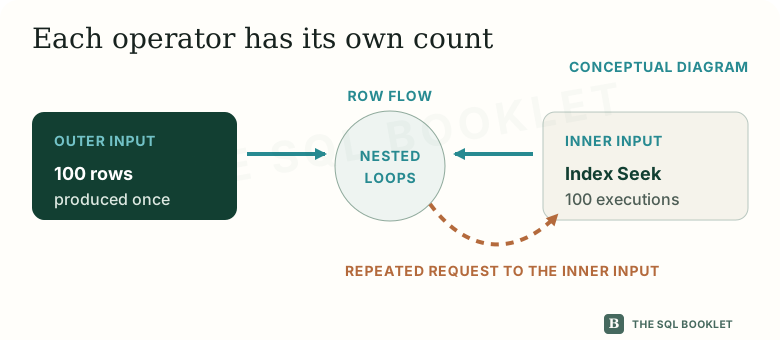
- 1Outer input
Supplies 100 rows to Nested Loops.
- 2Nested Loops
Requests the inner input once per row.
- 3Index Seek
Participates 100 times in this example.
The execution count tells us how many times the operator participated during the observed plan execution. It does not automatically represent how many users ran the query or how many times a stored procedure was called.
The outer input supplies the rows that begin each Nested Loops cycle. The inner input receives a new request to look for matches. If the outer input supplies 100 rows and one inner lookup occurs for each row, the inner operator can record 100 executions.
An operator can run repeatedly because another operator requests a new input. This commonly occurs on the inner side of Nested Loops: for every row from the outer input, the plan may request work from the inner input again.
Nested Loops names a join strategy. One input acts as the outer traversal and the other may be consulted repeatedly to find matches. A small operation can accumulate work when it repeats.
Read quantities with the same scope
Properties may distinguish rows per execution, rows accumulated across all executions, and data distributed among multiple threads. Before comparing two values, we must read their complete labels and confirm that they have the same scope.
If a field already says “all executions,” multiplying it by the execution count would duplicate the quantity. When the plan uses parallelism, we must also determine whether the view presents a total or a per-thread breakdown.
We therefore do not apply a formula merely because two labels look familiar. We first identify:
- whether the value is estimated or observed;
- whether it covers one execution or all executions;
- how many times the operator participated;
- whether the figure is aggregated or divided by thread.
How to interpret these signals
A thick arrow, a high percentage, or many executions identifies a place to ask questions; it does not prescribe a change. We still need to relate those signals to rows read, rows produced, predicates, duration, CPU, and query context.
Reducing one visual figure does not guarantee an improvement for the complete workload. A change may help one execution while harming other parameters, writes, or queries.
What this vocabulary lets us describe
With this vocabulary, we can describe a small plan without judging it: locate the root, follow its branches, explain what the arrows transport, and open properties to clarify rows and executions.
The next article groups operators by the function they perform. That map makes it possible to recognize a node’s role before examining its figures or deciding whether it warrants investigation.